ContactResumeResearchTeachingStudentsSoftwareAnimationMusic dark-mode: off

Seiler’s Interpolation

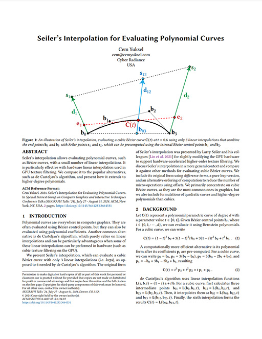
Above is an interactive demo showing a cubic Bézier curve with 4 control points b₀, b₁, b₂, and b₃ evaluated using Seiler’s interpolation, which uses 2 Seiler points s₁ and s₂ computed from the Bézier control points.

Abstract

Seiler's interpolation allows evaluating polynomial curves, such as Bézier curves, with a small number of linear interpolations. It is particularly effective with hardware linear interpolation used in GPU texture filtering. We compare it to the popular alternatives, such as de Casteljau's algorithm, and present how it extends to higher-degree polynomials.

Summary

For a cubic curve, its two Seiler points s₁ and s₂ can be computed from the Bézier control points b₀, b₁, b₂, and b₃ using

s₁ = 3b₁ – b₀ – b₃
s₂ = 3b₂ – b₃ – b₀

Then, the Bézier curve C at parametric position t can be evaluated with only 3 linear interpolation (lerp) operations using the end points of the Bézier curve and the two Seiler points:

b03	= lerp( b0, b3, t )
s12	= lerp( s1, s2, t )
C(t)	= lerp( b03, s12, (1–t)t )

Using this representation, one can store the Seiler points s₁ and s₂ instead of the internal Bézier control points b₁ and b₂. In a GPU implementation, these control points can be read from a texture, which can automatically perform the first two linear interpolations above in hardware, and only the final linear interpolation needs to be computed in software.

Publications